Physics4C thsiung: November 2011

There are three parts with this experiment. The first part is to look at the light spectra of white light through a grating. The second part is to look at an unknown gas to with a grating to determine the contents of the tube with spectra lines. Last, we compare the wavelength results to fix any systematic shift with an equation. After, we determine the possible wave lengths of the hydrogen gas tube.
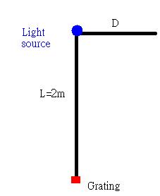
For the following experiment, the apparatus is

The value of the grating will be 1.67*10^-6 m
The equation to find the wavelength at distinct position is λ=(D*d)/√(L^2+D^2) where D is the spectra light's distance from the light source. L is the distance between the light source and the grating. d is the measurment of the grating.
We just look through the grating to determine the spectra lines.

1.
For experiment one, the light source will be white light (regular light bulb), and we measured the distance for the spectra light. Interesting thing about this experiment is that the light bulb has some diameter about 1.5cm;thus, we need to add this number to compensate the increase in the value of L(2.015m). By doing the experience we obtained the value of each spectra line (the midpoint of continuous spectra)

	Violet	Blue	Green	Yellow	Red
cm+-0.5cm	43.5	49.5	58.5	65	76

End points are 42cm &85.5cm

If we look only at the end points of the spectra lines, we range of the wavelength is gonna be 341nm~652nm±10nm

The results we got from doing the experiment is within the visible spectra, which is 380~750nm(according to wikipedia).

2. The second experiment is to determine the type of gas inside the tube we have

In this case, we do the same steps with just the white light to determine the spectra line ragnes are.

	Violet	Green	Yellow	Red
cm+-0.5cm	45.5~59	59~62.5	62.5~66.5	66.5~100

If we take the the midpoint of each region we get
Violet=52.25cm±0.25cm
Green=60.75cm±0.25cm
Yello=64.5cm±0.25cm
Red=66.5cm±0.25cm

If we calculated out the wavelength of each section
we get
Violet=422nm±4nm
Green=485nm+4nm
Yellow=513nm±4nm
Red=642nm+±4nm

If we match the spectra line we have to an known gas spectra, we will get the result similar to mercury gas.

3. Lastly, we use the same method the measure the four primary lines of the hydrogen gas spectrum.

The problem we had for this experiment is that our hydrogen gas tube has a leak;thus, the light that produced is really dean that we had trouble to do this experiment. At the end, we just worked with Christ and Eric to do the experiment and obtained the data from them.

	Violet/Blue	Green	Orange/Yellow	Red
cm+-2cm	46.5	50.6	62.1	70.8

And to fixed the systematic error they had the equation of λ_actual=1.051λ_exp+4.538

If we calculate the numbers, we will get
Violet/Blue=378nm±11nm
Green=410nm±11nm
Orange/Yello=495nm±11nm
Red=557nm±11nm

After the calibration, the actual result is

Violet/Blue=402nm±16nm
Green=435nm±16nm
Orange/Yello=525nm±16nm
Red=590nm±16nm

And if we compare to the actual results

Color	Frequency	Wavelength
violet	668–789 THz	380–450 nm
blue	631–668 THz	450–475 nm
cyan	606–630 THz	476–495 nm
green	526–606 THz	495–570 nm
yellow	508–526 THz	570–590 nm
orange	484–508 THz	590–620 nm
red	400–484 THz	620–750 nm

The results are fairly close to the actual number within their uncertainties.

Today, we had our first computer lab experiment that we get to have the chance to play with python. Unlike in 4A, this time we use from pylab import* in-order to generate graphing ability to present in the program. The three parts of this program are: generate sin graph, generate Gaussian graph, and last is to generate multiple sin graph and add them together with different period and amplitude. The amplitude of
each graphs will depend on the Gaussian function.
In-order for the program to work, we need to install pylab library into our computer, we can obtain the file from the link http://sourceforge.ent/projects/matplotlib/

Here is the code we had
_________________________________below is the code_________________________________
from pylab import*
harmonics= 20
center=harmonics/2
sigma=1
coeff=1/((sqrt(2*pi))*sigma)
gauss_list=[]
domain_list2=[]
L=10
knot= 2*pi/L
b_list=[]
kdomain=[]
##
##for k in arange(0,200,0.1):
##    bofk=(1/(knot))
##    b_list.append(bofk)
##    kdomain.append(k)
####plot(kdomain,b_list)
##

for x in range(1,harmonics):
    gauss=coeff*exp(-(x-center)**2/(2.*sigma**2))
    gauss_list.append(gauss)
    domain_list2.append(x)

##A_coeff_1=1
##wave_constant_1=1
##sine1_list=[]
##domain_list=[]
##for x in arange(-pi,pi,0.1):
##    sine1=A_coeff_1*sin(wave_constant_1*x)
##    sine1_list.append(sine1)
##    domain_list.append(x)
w=1
Fourier_Series=[]

for i in range(1,harmonics):
    sine_function=[]
    x=[]
    for t in arange(-pi,pi,0.01):
        sine_f=gauss_list[i-1]*sin(i*w*t)
        sine_function.append(sine_f)
        x.append(t)
    ##plot(x,sine_function)
    Fourier_Series.append(sine_function)

superposition=zeros(len(sine_function))
for function in Fourier_Series:
    for i in range(len(function)):
        superposition[i]+=function[i]
print kdomain
plot(x,superposition)
##plot(domain_list2,gauss_list)
##plot(domain_list,sine1_list)
show()
_________________________________End of the code_________________________________
Here are some of the results that we got

First this is the graph for jut plotting one sine function

After this is to plot the Gaussian function

At the end, we combine the since function with amplitude of the results from Gaussian function

Also, if we put more sine function (harmonics), the tails of the graph will be longer

After computing these results, we were ask few questions

Using the integral in $\psi(x)=\int_{0}^{\infty}B(k) \:{\rm cos}\: kx \: dk$ , determine the wave function $\psi \left( {x} \right)$ for a function $B\left( k \right)$ given by
$B\left( k \right) = \left\{ {\begin{array}{*{20}c} 0 & {k < 0} \\ {1/k_0 {\rm{,}}} & {0 \le k \le k_0 } \\ {0,} & {k > k_0 } \\ \end{array}} \right.$ .
This represents an equal combination of all wave numbers between 0 and k_0