Physics4C thsiung: Visualizing Wave Packets

Today, we had our first computer lab experiment that we get to have the chance to play with python. Unlike in 4A, this time we use from pylab import* in-order to generate graphing ability to present in the program. The three parts of this program are: generate sin graph, generate Gaussian graph, and last is to generate multiple sin graph and add them together with different period and amplitude. The amplitude of
each graphs will depend on the Gaussian function.
In-order for the program to work, we need to install pylab library into our computer, we can obtain the file from the link http://sourceforge.ent/projects/matplotlib/

Here is the code we had
_________________________________below is the code_________________________________
from pylab import*
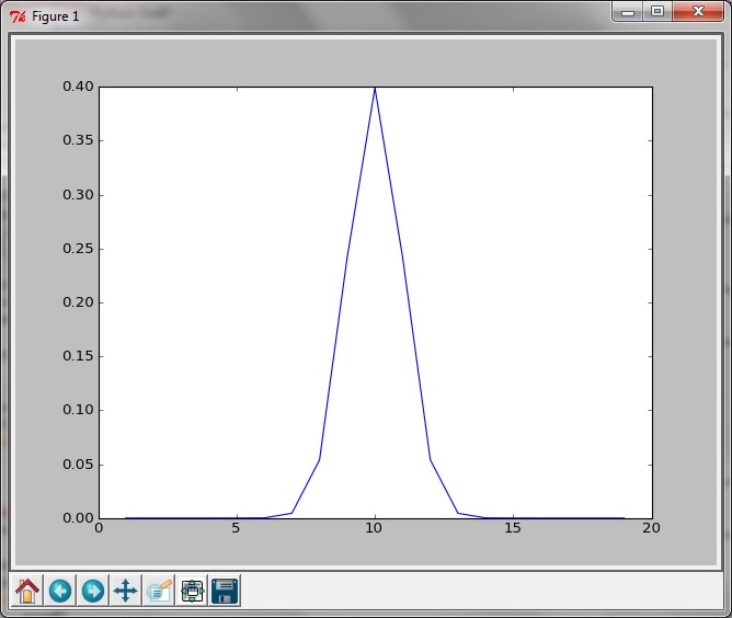
harmonics= 20
center=harmonics/2
sigma=1
coeff=1/((sqrt(2*pi))*sigma)
gauss_list=[]
domain_list2=[]
L=10
knot= 2*pi/L
b_list=[]
kdomain=[]
##
##for k in arange(0,200,0.1):
##    bofk=(1/(knot))
##    b_list.append(bofk)
##    kdomain.append(k)
####plot(kdomain,b_list)
##

for x in range(1,harmonics):
    gauss=coeff*exp(-(x-center)**2/(2.*sigma**2))
    gauss_list.append(gauss)
    domain_list2.append(x)

##A_coeff_1=1
##wave_constant_1=1
##sine1_list=[]
##domain_list=[]
##for x in arange(-pi,pi,0.1):
##    sine1=A_coeff_1*sin(wave_constant_1*x)
##    sine1_list.append(sine1)
##    domain_list.append(x)
w=1
Fourier_Series=[]

for i in range(1,harmonics):
    sine_function=[]
    x=[]
    for t in arange(-pi,pi,0.01):
        sine_f=gauss_list[i-1]*sin(i*w*t)
        sine_function.append(sine_f)
        x.append(t)
    ##plot(x,sine_function)
    Fourier_Series.append(sine_function)

superposition=zeros(len(sine_function))
for function in Fourier_Series:
    for i in range(len(function)):
        superposition[i]+=function[i]
print kdomain
plot(x,superposition)
##plot(domain_list2,gauss_list)
##plot(domain_list,sine1_list)
show()
_________________________________End of the code_________________________________
Here are some of the results that we got

First this is the graph for jut plotting one sine function

After this is to plot the Gaussian function

At the end, we combine the since function with amplitude of the results from Gaussian function

Also, if we put more sine function (harmonics), the tails of the graph will be longer

After computing these results, we were ask few questions

Using the integral in $\psi(x)=\int_{0}^{\infty}B(k) \:{\rm cos}\: kx \: dk$ , determine the wave function $\psi \left( {x} \right)$ for a function $B\left( k \right)$ given by
$B\left( k \right) = \left\{ {\begin{array}{*{20}c} 0 & {k < 0} \\ {1/k_0 {\rm{,}}} & {0 \le k \le k_0 } \\ {0,} & {k > k_0 } \\ \end{array}} \right.$ .
This represents an equal combination of all wave numbers between 0 and k_0